Methodology

Research Design

The Effect of Particulate Pollution on Life Expectancy

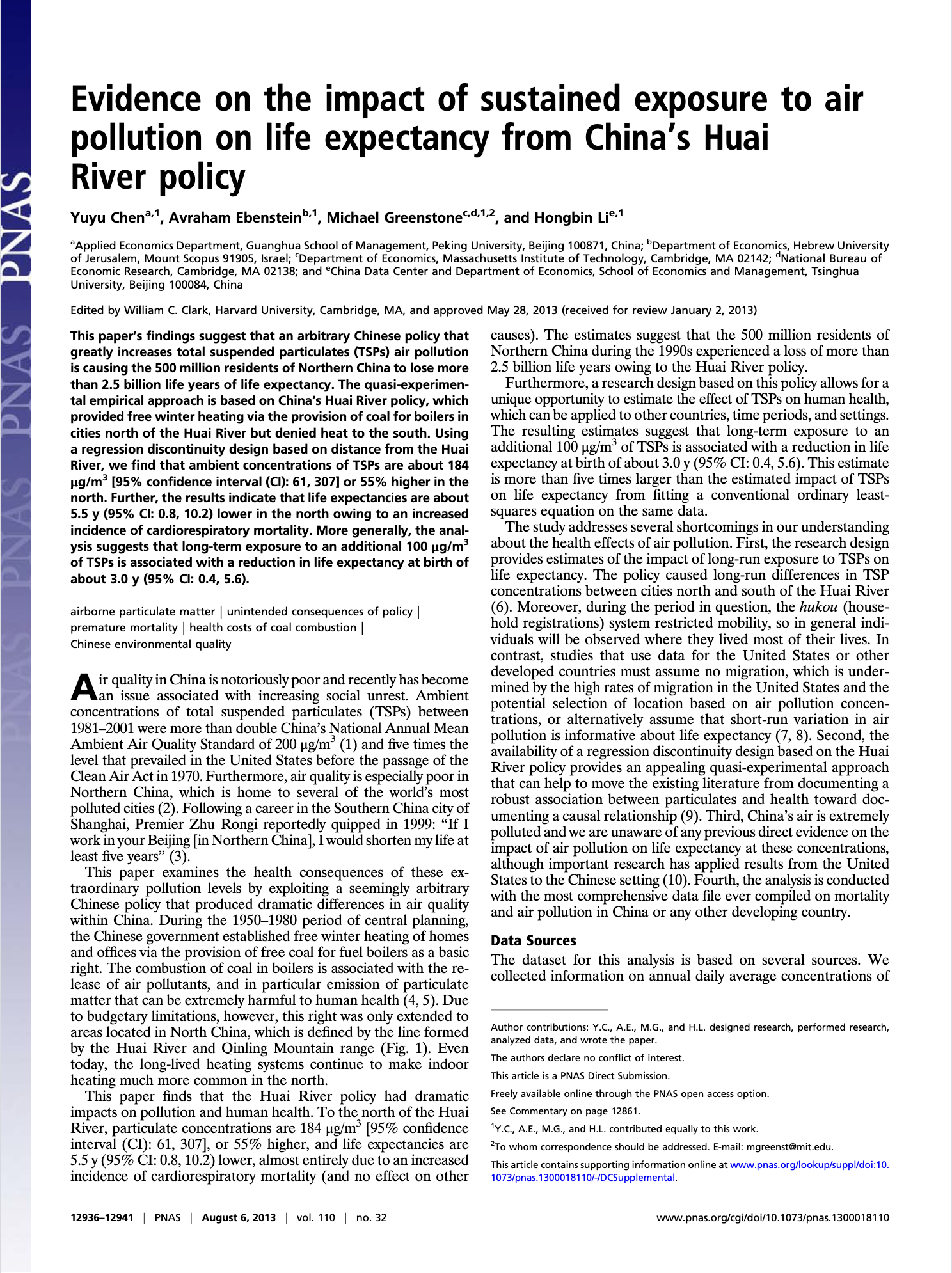
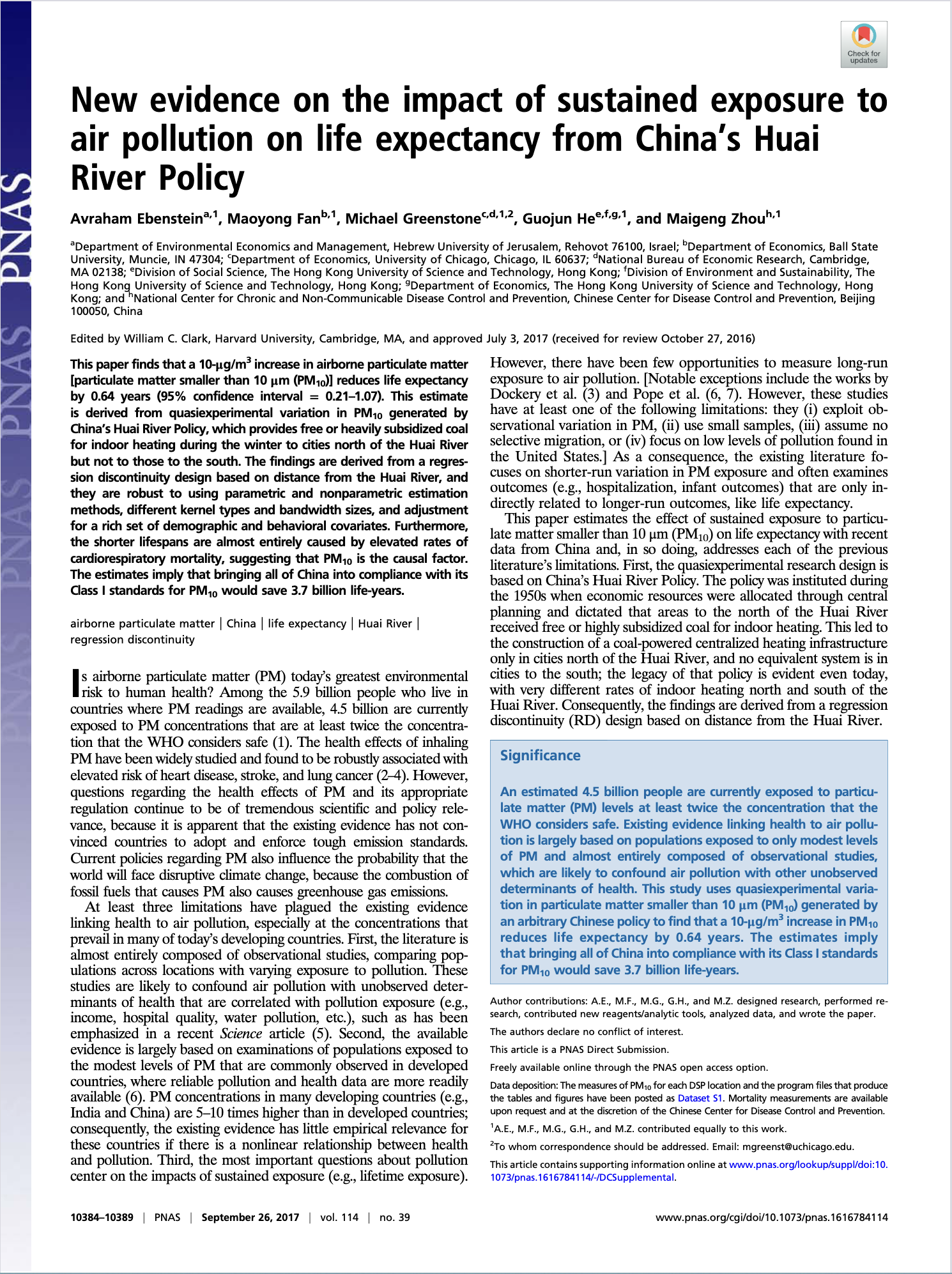
The AQLI is based on a study by Michael Greenstone, Avraham Ebenstein, Maoyong Fan, Guojun He, and Maigeng Zhou (2017) that, thanks to a unique social setting, were able to measure the effect of sustained exposure to high levels of pollution on a person’s life expectancy.

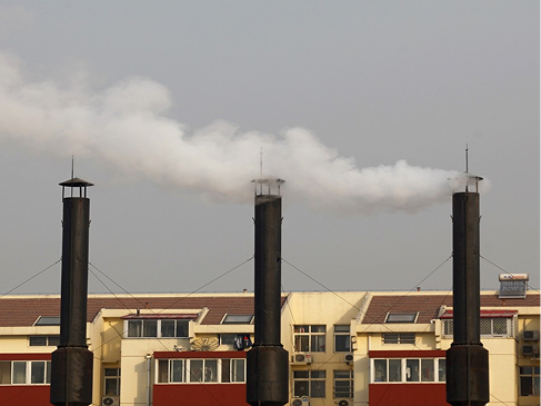
In China, areas in the north have traditionally experienced higher levels of pollution in part because of a government policy initiated during the planning period (i.e., 1950 to 1980) that gave those living north of the Huai River, where it is colder, free coal to power boilers for heating. While the policy’s purpose was to provide warmth in the winter to those who needed it the most, it resulted in a high and differential reliance on coal north of the Huai River, relative to the south. The legacy of the policy remains today, with very different rates of indoor heating north and south of the Huai River as the north continued to rely on the coal heating systems. At the same time, the hukou household registration system discouraged people from leaving the communities where they were born. This effectively meant that people exposed to particulate pollution could not migrate to areas with cleaner air. Combined, these two policies created a unique demarcation line where the researchers were able to study the impact of high levels of pollution over.

The more recent of the pair of studies indicates that sustained exposure to an additional 10 μg/m³ of PM10 reduces life expectancy by 0.64 years.[3] Although the study was based solely on a Chinese setting, together, the regions and years covered in the study saw a wide range of pollution levels: in the areas within five degrees latitude of the Huai River, the range of PM10 levels within a standard deviation of the mean is 75-148 μg/m³ of PM10 (approximately equal to 48-96 μg/m³ of PM_2.5). The full range within five degrees latitude of the river is 27-307 μg/m³ of PM10 (approximately equal to 18-200 μg/m³ of PM_2.5). Thus, the relationship between life expectancy and particulate pollution that underlies the AQLI is derived from a PM_2.5 distribution similar to the observed global distribution, providing a credible basis for generalizing the measured pollution-life expectancy relationship from Ebenstein et al. (2017).

Figure: PM₁₀ Concentrations in China and the Huai River Dividing Line in Ebenstein et al. (2017)

---

WHO Guideline and National Standards for PM_2.5:

The AQLI measures potential gains in life expectancy by lowering PM_2.5 concentrations to meet either the WHO guideline for particulate matter concentrations or nationally administered air quality standards (National Standards). The WHO’s guideline is 5 micrograms per cubic meter (μg/m³), which corresponds to the lowest level of long-term exposure that the WHO found to raise mortality with greater than 95% confidence.[1]

With an abundance of scientific evidence on the negative health impacts of particulate pollution exposure, even at relatively low concentrations, on September 22, 2021 the World Health Organization (WHO) updated its guidance on the acceptable level of particulate pollution people should breathe.[2] The update, from 10 μg/m³ to 5 μg/m³ , was the first since establishing air quality guidance in 2005. The WHO’s decision to revise its guideline by such a significant amount is a powerful signal that air pollution is more deadly than initially thought.

Country-specific nationally administered annual standards were identified for 83 countries and range from 8–40 μg/m³ .[3] For the remaining countries for which we could not identify a national standard, we indicate on the map tool that they lack a national PM₅ standard and do not calculate gains in life expectancy relative to national standard. Additionally, the AQLI allows users to enter their own percent reduction in pollution concentrations and see the gains in life expectancy that would result.

---

Estimating Life Expectancy Gains by Meeting National Standard or WHO Guideline

To use the results of Ebenstein et al. (2017) in building the AQLI, we first convert to PM_2.5. Due to data availability constraints, Ebenstein et al. (2017) measure the impact of particulate pollution on life expectancy in terms of levels of PM10, particles smaller than 10 micrometers in diameter. Since global air pollution data only measure PM_2.5, the most harmful type of particulate pollution, we convert the study’s estimates to units of PM_2.5 using a 0.65 PM_2.5-to-PM₁₀ ratio, which closely aligns with conditions in China during the time period of the study.[5] This translates to:

In other words, life expectancy is reduced 0.98 years per 10 μg/m3 of sustained exposure to PM_2.5.

Following the epidemiology literature, the AQLI assumes a linear relationship between long-term exposure to PM_2.5 and life expectancy throughout the observed PM_2.5 distribution.[6] Though it is possible that the pollution-life expectancy relationship is nonlinear over certain ranges of PM_2.5 concentrations and/or that there is a threshold below which PM_2.5 has no effect, Therefore, to estimate the potential gain in life expectancy within each grid-cell, the AQLI increases the loss in life expectancy by 0.98 years for every 10 μg/m³ of additional long-term exposure above the reference standard (either the WHO guideline or national standard, or a user entered standard).

For both pollution concentrations and loss in life expectancy, the AQLI aggregates grid-cell-level estimates to national and sub-national administrative boundaries. Aggregations are population-weighted. For example, in 2020, the annual average PM_2.5  level in Beijing was 38 μg/m³, and the level in Guangzhou was 23 μg/m³. When calculating China’s national 2020 annual average PM_2.5 level, Beijing’s PM_2.5 level is given about 50% more weight than Guangzhou’s, because Beijing’s population is about 1.5 times that of Guangzhou. Thus, China’s national average PM_2.5 level of 32 μg/m³ means that on average, each person in China was exposed to an annual average PM_2.5 level of 32 μg/m³ in 2020. These aggregated values are what is shown in the map tool at the national and sub-national levels.

---

Grid-Level Particulate and Population Estimates

Reliable, geographically extensive pollution measurements are critical to understanding the extent of air pollution and its health impacts. Unfortunately, many areas around the world currently lack extensive pollution monitoring systems. Of the areas with monitoring, many are either newly established or did not begin monitoring PM_2.5 until recently, making it impossible to track long-term impacts. The quality and trustworthiness of reported monitor data also varies, compromising comparisons of pollution across regions.

To construct a single dataset of particulate pollution and its health impacts that is global in coverage, local in resolution, consistent in methodology, and that spans many years to reveal pollution trends over time, the AQLI incorporates satellite-derived annual ambient particulate pollution (PM_2.5) concentration estimates spanning 24 years from 1998-2021. This data, constructed by Donkelaar et al. (2021), covers the globe at a certain given set of resolutions. As a hypothetical example, at the resolution of 0.05° x 0.05° the surface of the Earth is divided into grid cells no bigger than 6 km x 6km, or what is 1/30 the size of New York City, 1/60 the size of Delhi, or 1/170 the size of urban Beijing. For each year, the dataset provides the PM_2.5 concentration over each of these grid cells. As the resolution of the data increases, the grid cell size gets smaller, providing a more finer-grained view of the pollution landscape. This year AQLI reports the data at a resolution of 0.01° Lat x 0.01° Long.

How is it possible to know the PM₅ concentration in areas with sparse or even a complete lack of pollution monitors? Donkelaar et al. (2020) uses a three-step process.

1. From satellites, they obtain measurements of aerosol optical depth (AOD) over each grid cell. Particles in the air block sunlight, so heavier air pollution means less light can go through the atmosphere. AOD is a unitless measure of how much light passes through the vertical column of air over a grid cell.
2. To convert AOD to PM_2.5, they employ a widely-used model called GEOS-Chem. The inputs to this model are meteorological data and data on emissions of numerous compounds including PM, SO2, NOx, and volatile organic compounds (the latter three are gases that form PM upon being emitted into the atmosphere). Using these inputs, the model simulates the relationship between AOD and PM_2.5 across space and time. Combining the GEOS-Chem simulation with satellite-derived AOD measurements yields a preliminary global gridded PM_2.5 dataset.
3. To further improve accuracy, they calibrate this dataset with PM_2.5 readings from available ground-level monitors using a Geographically Weighted Regression (GWR). That is, for grid cells lying close to monitors, they calculate how geophysical factors such as aerosol composition and distance to urban areas affect the deviation of the satellite-derived PM_2.5 from monitor readings. This allows them to estimate how much the satellite-derived PM_2.5 deviates from ground truth even where there are no monitors, and to adjust accordingly. Furthermore, their latest paper (Donkelaar et al. 2021, i.e. V5.GL.02) follows the methodology of their previous paper, but updates the ground-based observations used to calibrate the geophysical PM_2.5 estimates for the entire time series, and extends temporal coverage through 2020.

The resulting dataset is highly consistent with available ground-level monitor data (R2=0.92 in cross-validation with out-of-sample monitors).

The AQLI uses a version of this satellite-derived PM_2.5 dataset that excludes mineral dust and sea salt. Thus, our data can be interpreted as concentrations stemming primarily from human activity (such as automobile emissions, power plants, or industrial activities) rather than natural sources. This allows us to focus on the subset of particulate pollution which has a more similar composition to the particulates studied in Ebenstein et al. (2017) that predominantly relies on variation due to difference in coal combustion, and which can be most easily targeted by public policies.

The AQLI uses population data from the 2019 LandScan Global Population Database, which uses spatial methods to disaggregate census population counts in each country into grid cells of length 30 arc-seconds. These grid cells are about 1 km2 around the Equator, and smaller elsewhere. After combining the detailed population data with the satellite estimates of PM_2.5 concentrations, the result is a global gridded database of ambient PM_2.5 concentrations with associated population counts. The population counts are used as weights when aggregating PM_2.5 concentrations and life expectancy results from the grid level up to the local, state, national, and global averages.

When aggregating pollution and life expectancy gains for any year, the AQLI uses the 2019 population data.

The AQLI is updated each year with the latest available PM_2.5 data.

Evolution of Satellite Derived PM2.5 data

Data Update

Reliable, geographically extensive pollution measurements are critical to understanding the extent of air pollution and its health impacts. Unfortunately, many areas around the world either lack extensive pollution monitoring systems or did not begin monitoring PM_2.5 until recently, making it impossible to track long-term global trends. To construct a single dataset of particulate pollution and its health impacts that is global in coverage, local in resolution, consistent in methodology, and that spans many years to reveal pollution trends over time, the latest AQLI data incorporates satellite-derived annual ambient PM_2.5 concentration estimates spanning 24 years from 1998-2021 by the Atmospheric Composition Analysis Group at the University of Washington (methodology described in van Donkelaar et al. (2021). The latest raw dataset (version: V5.GL.03) is publicly accessible at: https://sites.wustl.edu/acag/datasets/surface-pm2-5/. The AQLI uses a version of this data that excludes sea salt and dust.

There are differences between the satellite-derived PM_2.5 dataset used in this report and those used in previous AQLI reports. For example, in the new and revised 2021 dataset used this year, the estimated global population-weighted average PM_2.5 concentration for the year 2019 has been revised upwards relative to the 2020 dataset used in our 2022 AQLI update, from 27.7 to 28.5 µg/m³ (Figure A.1).

According to van Donkelaar et al. (2021), satellite-derived PM_2.5 data were constructed by converting measurements of aerosol optical depth (AOD) over each grid cell into PM_2.5 measurements using a chemical transport model called GEOS-Chem. These estimates were then subsequently calibrated to regional ground-based observations of both total and compositional mass using a Geographically Weighted Regression (GWR). Over time, improvements in the model and calibration inputs, alongside growing ground level monitoring coverage necessitate periodic updates to the historical PM_2.5 dataset.

In the figure below, we plot and compare the global population-weighted PM_2.5 -time trends using various years’ versions of the annual average PM_2.5 dataset. Although the new and revised PM_2.5 dataset yields global average concentration levels that are higher on average than those estimated using the 2020 and 2016 reference datasets and lower on average than the 2019 reference dataset, the overall picture remains the same. The global annual average PM_2.5 level has shifted between 3.8 to 7.2 times the WHO guideline, making air pollution making air pollution the greatest external threat to human health globally.

 

Note: The “2021 dataset” line plots the global population-weighted annual average PM_2.5 trend using data accessible from https://sites.wustl.edu/acag/datasets/surface-pm2-5/ (V5.GL.03) and methodology described in van Donkelaar et al. (2021). The “2020 dataset” line plots the global population-weighted average PM_2.5 trend using data from van Donkelaar et al. (2021). The “2019 dataset” line plots the analogous trend using data from Hammer et al. (2020). The “2016 dataset” plots the trend using data from van Donkelaar et al. (2016). Note that the AQLI uses a version of all datasets that excludes sea salt and dust. To learn more about these versions, visit: https://sites.wustl.edu/acag/datasets/surface-pm2-5/.

 

Why is AQLI’s pollution data different from what local monitors tell me?

Users may find that the AQLI’s satellite-derived pollution data differs from what their governments or local air quality monitors report. Some of the discrepancies are by design, reflecting differences in the operational definition of particulate pollution level:

• Dust and sea salt. Whereas monitors pick up all kinds of particulates, the AQLI intentionally uses raw PM_2.5 data from which the shares of mineral dust and sea salt have been removed in order to target human-caused pollution. This decreases the AQLI’s reported pollution, especially in arid regions such as North Africa, the Middle East, Sub-Saharan African, and northwestern China.
• Area average vs. point estimates. The satellite-derived raw PM_2.5 data that AQLI uses measures the average air pollution within each block of a grid at a given set of resolutions. For example, a 05 x 0.05 degree grid  is about 6 x 6 km at the equator, and smaller towards the poles. In contrast, air pollution monitors are located at single points – e.g. 100m downwind of the brick kiln, or in a tree in the park. They measure the air pollution level at their specific point locations, and the average of their measurements could be higher or lower than the average pollution level in the entire area.
• Area average vs. point estimates. The satellite-derived raw PM_2.5 data that AQLI uses measures the average air pollution within each block of a 0.05 x 0.05 degree grid (about 6 x 6 km at the equator, and smaller towards the poles). In contrast, air pollution monitors are located at single points – e.g. 100m downwind of the brick kiln, or in a tree in the park. They measure the air pollution level at their specific point locations, and the average of their measurements could be higher or lower than the average pollution level in the entire area.
• Population weights. Assuming that the raw pollution data is at the resolution of a 0.05 x 0.05 degree grid, and there are generally multiple such grid blocks within a political jurisdiction (e.g. county, district, prefecture). To show the particulate pollution and life expectancy impact experienced by each person, on average, within a local or national jurisdiction, the AQLI aggregates grid-level data using population weights. This means that, for example, if a county consists of a large, low-pollution city and a small but highly polluted industrial town, the AQLI’s numbers for that county more closely reflect the cleaner air experienced by the city-dwellers who make up most of the county’s total population. In such a case, the AQLI does not imply that air pollution has little health consequences for everyone in the county. In general, the grid-level satellite-derived pollution dataset created by Donkelaar et al. (2020) is quite consistent with ground-level monitor measurements (R2 = 0.92 with monitor measurements that were used to calibrate the satellite-derived dataset). However, under special geographical circumstances, the satellite measurements may not accurately reflect the pollution experienced by the local population.
• Resolution.
  • Although the 0.05 x 0.05 degree grid is a quite fine resolution for a global air pollution dataset, if an area has steep gradients of both pollution and population density at a scale below 0.05 x 0.05 degrees, this can result in mischaracterization of the pollution level experienced by the local population.
  • An extreme example of this is the case of Ulaanbaatar, Mongolia. The city’s oblong shape and location in the Tuul River Valley means that each grid block used to calculate the city’s aggregate pollution level also contains parts of the mountains that surround the urban valley area. Although air pollution is high in the urban area, air is much cleaner in the mountains. Since the average pollution level in every grid block is made lower by the mountains, population-weighting does not decrease the weight of less-polluted mountain areas.
  • The result is a much lower level of particulate pollution and resulting life expectancy impact for the city as a whole than what monitor data would tell us. For example, air pollution monitors measured an annual average PM_2.5 of 92 μg/m³ in 2016, whereas the AQLI calculates that it was 19 μg/m³. In this case, the former is more indicative of the quantity of particulates entering Ulaanbaatar residents’ lungs. In general, this is a potential issue for local areas in which pollution and population vary greatly, such as caused by a metropolitan area’s proximity to large mountains.
  • However, Ulaanbaatar is an extreme case in terms of the magnitude of the resulting discrepancy, due to the special combination of the jurisdiction’s size and shape, the steep pollution gradient within the jurisdiction, and the way that the satellite grid is placed over the jurisdiction.

---

Comparisons with Other Mortality Causes and Risks

Based on the AQLI’s results, if 2021 levels of ambient particulate pollution are sustained around the world, the life expectancy of everyone alive today would be on average 2.3 years lower than if particulate concentrations everywhere complied with the WHO guideline. In Pollution Facts, we compare this finding with the life expectancy impacts of other causes and risks of premature death. We do so using life tables, the same epidemiological approach that the Huai River studies used to calculate the relationship between particulate pollution and life expectancy.

A summary of this approach is as follows. From the WHO, we obtain the latest available (2019) life table of mortality data such as probability of death and life expectancy remaining for each sex and age interval 0-1, 1-4, 5-9, …, 80-84, and 85+.[7] We call these the “baseline” data. From the Global Burden of Disease (GBD)[8], for a variety of causes and risks of mortality (e.g. smoking, malaria), we obtain the rates of death in 2019   (again, the latest available as of March 2023 ) due to that cause or risk within each sex and age interval 0-1, 1-4, 5-9, …, 75-79, and 80+. For both of these data sets, we aggregate the highest age intervals into a single 80+ interval for consistency.

Now, using the baseline life table and following the procedure first outlined by Greenwood (1922) and Chiang (1984), we calculate average life expectancy for a male and a female born in 2019, assuming that mortality risks in each age interval remain constant into the future. Using the 2019 sex ratio at birth, we take a weighted average to aggregate the life expectancies by sex into a single average baseline life expectancy.[9]</9> This number accounts for the life expectancy impacts of all mortality causes and risks, based on their actual burdens in 2019.

To calculate what life expectancy at birth would hypothetically have been if a particular condition (e.g. smoking or malaria) did not exist, we subtract rates of death due to that condition from the life table baseline rates, then follow the same procedure as above to obtain the counterfactual average life expectancy at birth. The difference between the baseline life expectancy and this counterfactual life expectancy is the life expectancy impact of that condition, which we compare to the AQLI’s result of 2.2 years.

To do a country-specific comparison, country-specific life tables and mortality data are used. The data and code that produced these calculations can be found here.

______________________________

[1] WHO, 2021

[2] E.g., Burnett and Aaron, 2020.

[3] Many national standards were identified from Kutlar et al. (2017)

[4] Chen et al., 2013; Ebenstein et al., 2017

[5] The ratio of 0.65 is based on a careful review of studies that report historical PM_2.5-to-PM₁₀ ratios in China during a similar timeframe as Ebenstein et al. (2017). Two nationally representative studies are of particularly interest. Wang et al. (2015) measures PM_2.5-to-PM₁₀ ratios at 24 monitoring stations across the country between 2006 and 2014 and reports total averages by station/city. A back of the envelope population weighted-average calculation using these averages indicates a PM_2.5-to-PM₁₀ ratio of 0.73. Importantly, the list of cities in this study does not include some major metropolitan areas (e.g. Beijing), although many surrounding areas are included. Zhou et al. (2015) compiles a comprehensive nationwide database of all published literature (128 articles) which studied PM_2.5 and PM₁₀ mass concentrations from 1988 – 2010 and finds a PM_2.5-to-PM₁₀ ratio of 0.65 based on 589 pairs of data covering 57 cities and regions. Finally, we also considered the mass ratio PM_2.5/PM₁₀ of 0.66 used by the World Health Organization for China in its ambient pollution database. Given the comprehensiveness of Zhou et al. (2015) and how close its findings are to the WHO value (0.65 versus 0.66), we use 0.65 as the baseline PM_2.5-to-PM₁₀ ratio for the AQLI.

[6] See, for example, Global Burden of Disease (2017).

[7] WHO, 2019

[8] To date, the most updated data on Global Burden of Disease is from 2019.

[9] Sex Ratio at Birth, The World Bank; https://data.worldbank.org/indicator/SP.POP.BRTH.MF